Parametric Integration
Neil Trivedi
Teacher

Parametric Integration
Sometimes, a curve is not given in the usual form . Instead, both and are written in terms of a third variable, usually . This is called our parameter. So, when we want to evaluate an integral in the form
It is difficult because is not in terms of . So, in cases like these, we use parametric integration.
Parametric integration is the method we use to convert an integral such as , which involves , into an integral involving the third parameter. We do this by rewriting the integral in terms of the third parameter and then integrating as normal. This is pretty much the exact same as substitution.
Parametric Integration
Evaluating
when given parametric equations
1) Express in terms of . We differentiate with respect to to get . Then, we rearrange to isolate .
2) Rewrite the integral in terms of . We substitute and to give
3) If the integral is definite, change the limits from to . We use the equation to find which values of correspond to the original limits.
4) After the substitution and changing of the limits, we integrate as normal but with respect to instead of .
Example 1:
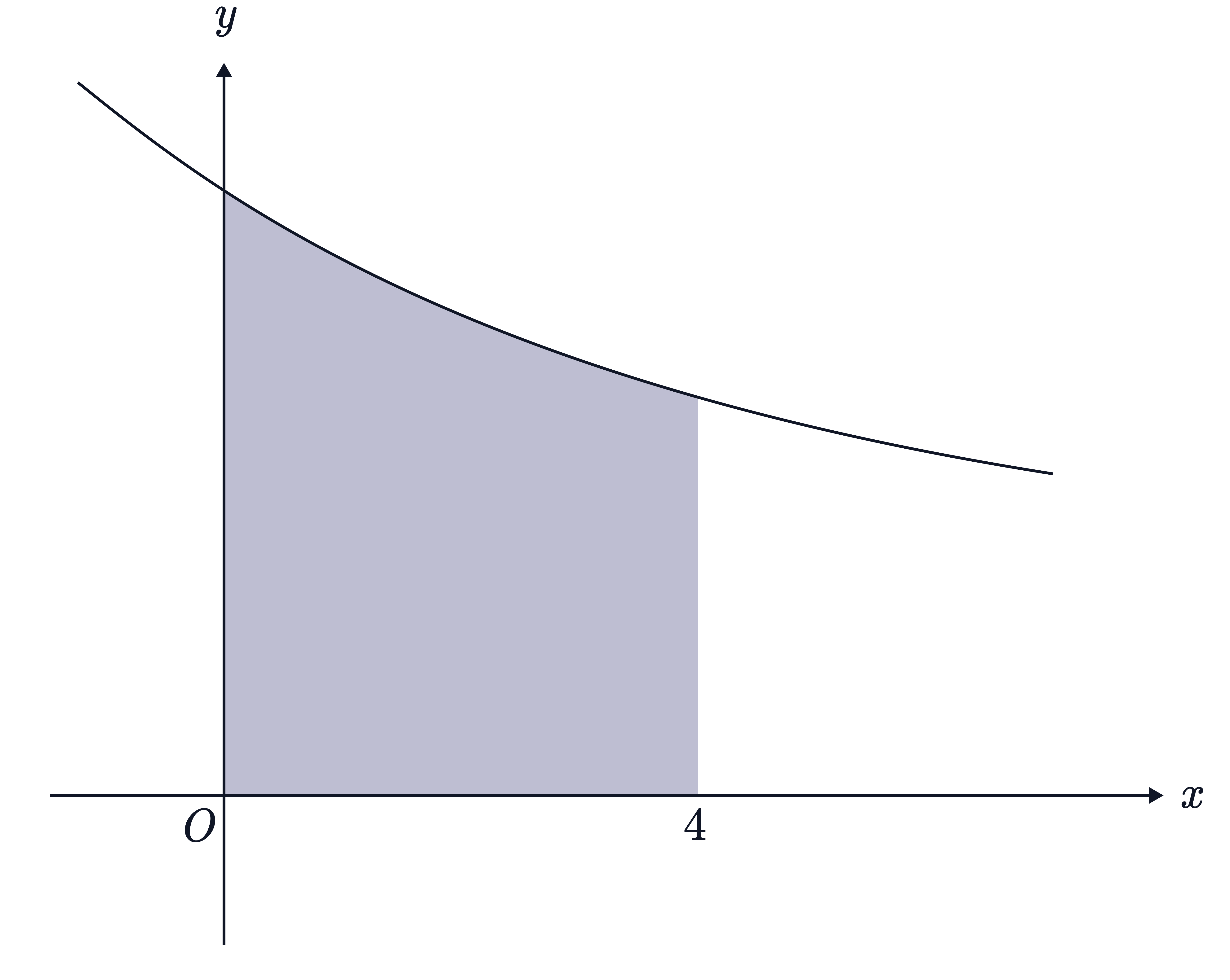
The diagram shows part of the curve with parametric equations
The shaded region is bounded by the curve, the coordinate axes and the line .
a) Find the values of the parameter when and when .
Single Step: Form two equations where and and solve for in each case.
b) Find the area of the shaded region.
Always start off by writing the area under the curve in Cartesian form.
Step 1: Like in substitution, we always change first. We want dt so we will find and rearrange for .
We differentiate the equation with respect to .
Rearranging to isolate ,
Step 2: Rewrite the integral.
We substitute and into the integral to rewrite it in terms of .
We already found our limits in part (a), so we replaced the limits right away.
The is a multiplier so we can write it outside.
Step 3: Integrate with respect to and evaluate the limits.
With integration by recognition, integrates to . We now evaluate the limits to find the exact area under the curve.
Using the logarithmic rule which states that .
No answer provided.
Example 2:
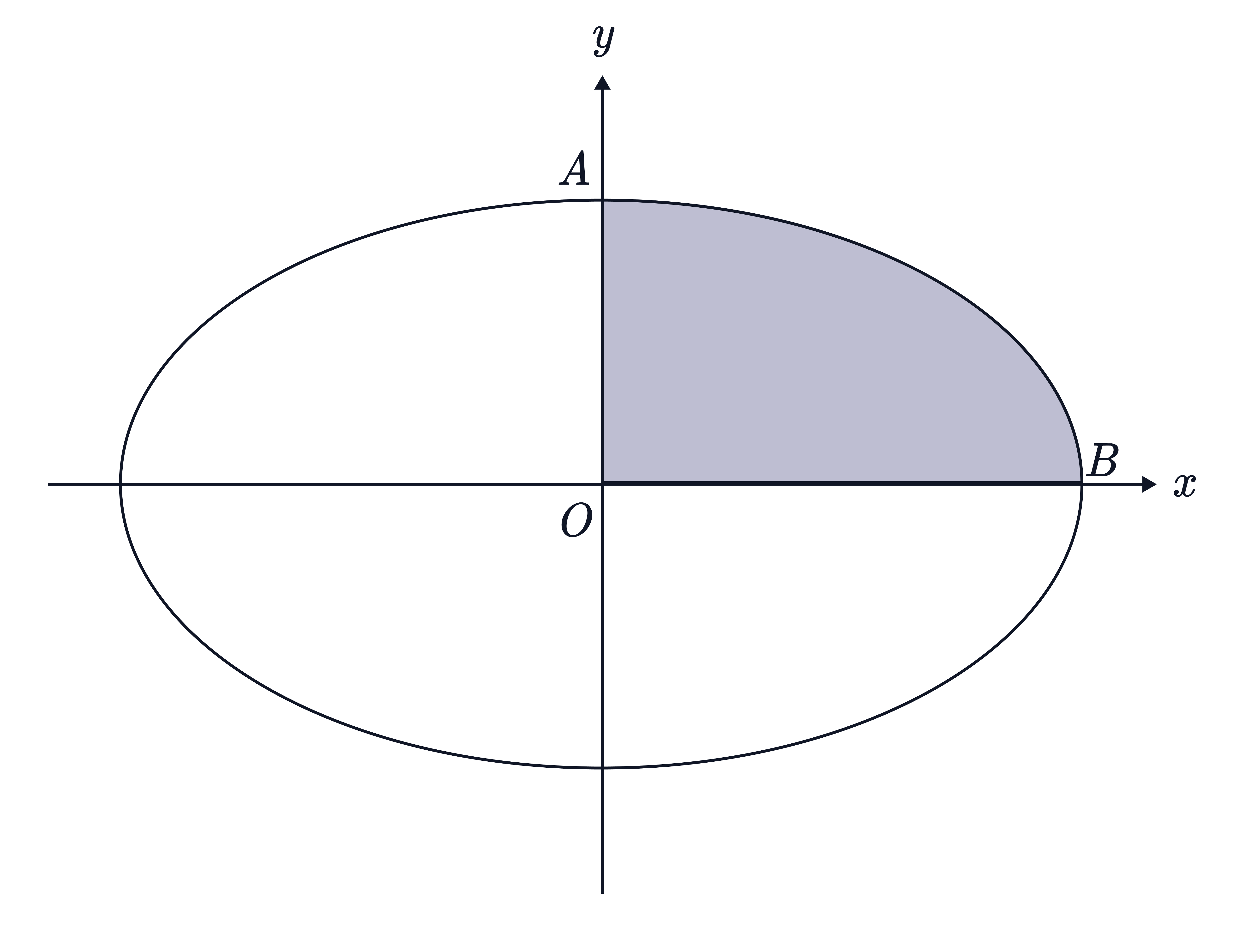
The diagram shows an ellipse with parametric equations
which meets the positive coordinate axes at and .
a) Find the value of the parameter at and .
Single Step: Form two equations where and and solve for in each case.
At point , .
Find the PV by applying the inverse function of .
(PV)
Trigonometric Functions | Finding the SV |
| PV |
| PV |
| PV |
Find the SV by working out PV
PV (SV)
There are no other values in the range so we can stop here. So, we have
We now substitute both values of into the equation and see which one corresponds to a positive coordinate because is in the positive axis.
When ,
When ,
We see that gives us a positive coordinate so at .
Now, we do the same for point . At , .
Find the PV by applying the inverse function of sin.
(PV)
Find the SV by working out PV
PV (SV)
There are no other values in the range so we can stop here. So, we have
We now substitute both values of into the equation and see which one corresponds to a positive coordinate.
When ,
We see that gives us a positive coordinate so at .
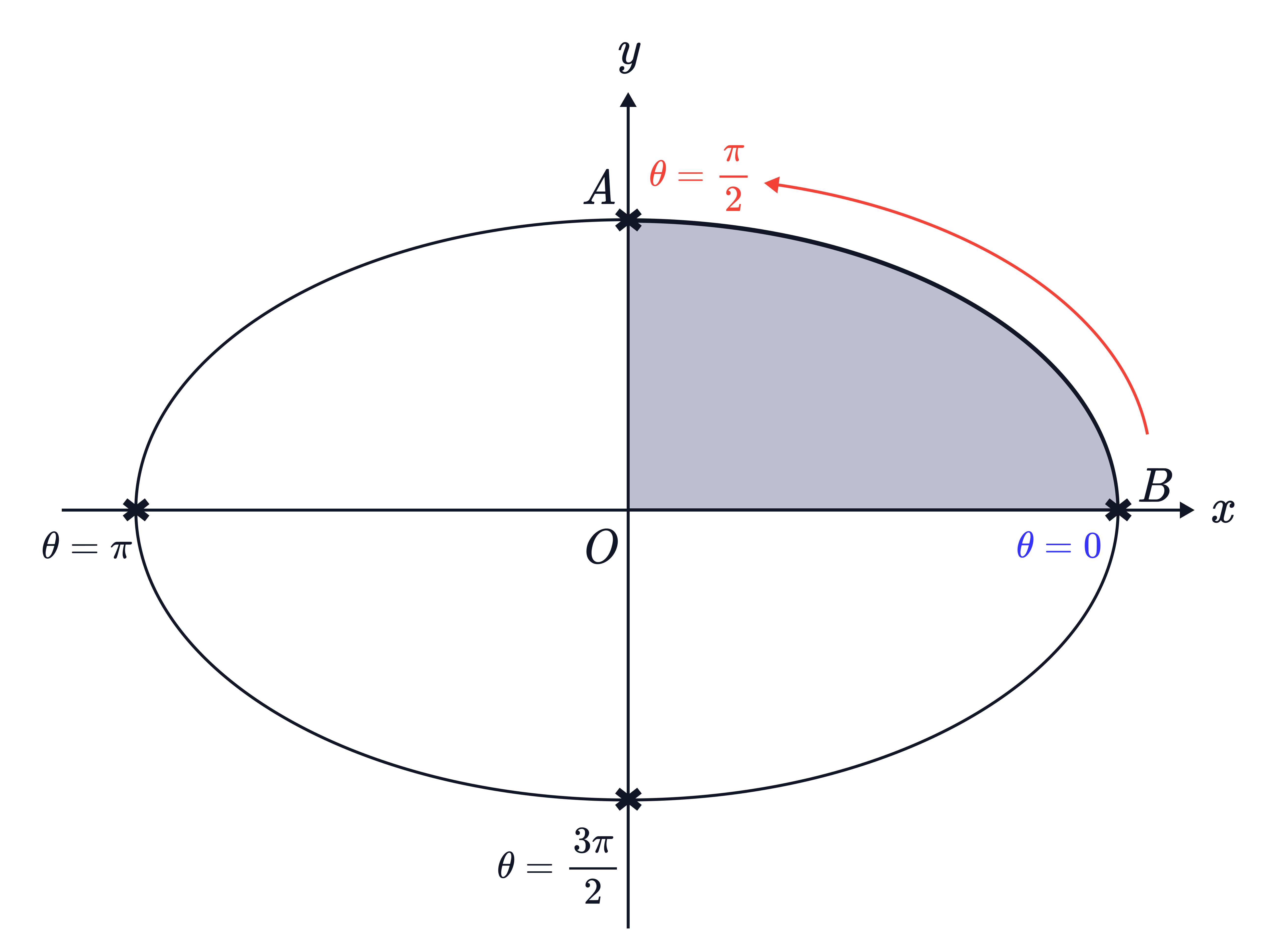
We can see our solutions for on this diagram, where and correspond to the positive and axes, respectively while our other two solutions, and correspond to the negative and axes, respectively.
We can also note that that as goes from to , we’re moving in an anti-clockwise motion, and once we’re at , it cycles. This is because the and graphs cycle every .
b) Find the area of the shaded region, and hence, find the area enclosed by the ellipse.
Always start off by writing the area under the curve in Cartesian form.
Step 1: Express in terms of .
We differentiate the equation with respect to .
Rearranging to isolate ,
Step 2: Rewrite the integral.
We substitute and into the integral to rewrite it in terms of .
Notice how when we changed our limits over to , the smaller limit is on top. The reason this is happening is because as increases, we are moving anti-clockwise (see diagram) which means we are integrating from right to left. However, we integrate from left to right. We can easily adjust our integral by multiplying what is inside our integral by and switching the limits.
The is a multiplier so we can write it outside.
Step 3: Integrate with respect to and evaluate the limits.
Firstly, we need to rewrite using a trigonometric identity because we cannot integrate it directly using recognition. For more, see our Integration using Trigonometric Identities note.
We’ll use the double angle formula for .
Rearranging for ,
Therefore,
Factorising out ,
We know that will integrate to . We make a guess as to what function may differentiate to get . We’ll guess . This angle is which differentiates to , then differentiates to , then the angle is kept the same.
Angle stays the same
Differentiated angle
Our guess differentiates to give , but we wanted . So, we multiply both sides by the constant we want over the constant we have, which will be .
Combining the terms,
Evaluating the limits, we get
No answer provided.
Challenging Question