The Z-Distribution
Neil Trivedi
Teacher

The Z-Distribution
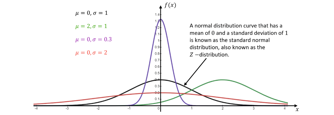
Sometimes, we may get normal distribution questions where we don’t know what the mean and standard deviation are. For these, we must use transformations to turn our distribution into the standard normal distribution, which has a mean of and a standard deviation of . We call this the Distribution where .
Here are some normal distribution curves and we can see how they compare to a standard normal distribution curve. We can observe that the “wider” curves have a larger standard deviation.
Suppose we are observing the event and are asked to apply some calculations to it. Currently, we can’t because we cannot input unknown means and standard deviations into our calculator.
Suppose we want to find . We need to apply some transformations to ensure we can use the calculator; this is because we will know what the mean and standard deviation are.
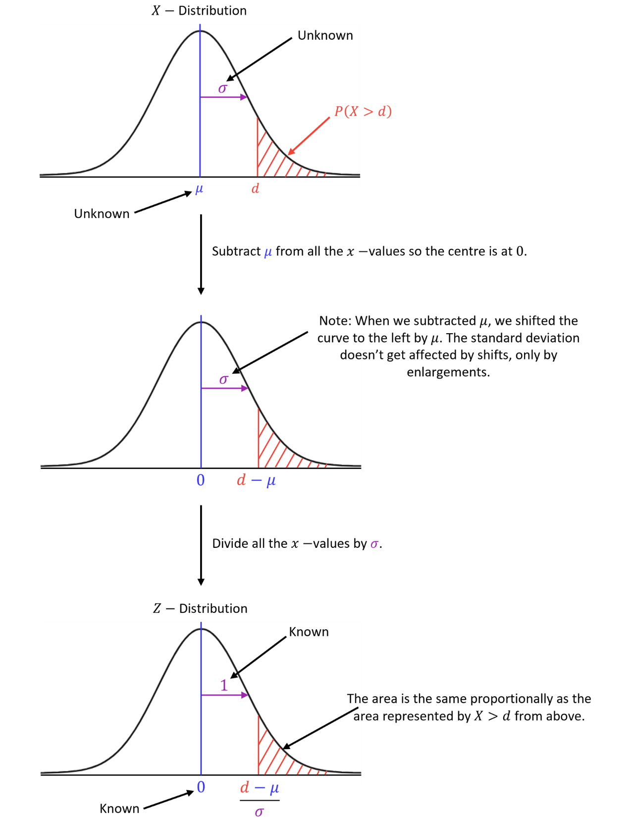
To go from to , we apply the transformation of
Notation to be familiar with for the Distribution:
is the cumulative distribution for the standard normal distribution.
Example 1:
The random variable . Write the following in terms of for some value of .
a)
Single Step: Apply the transformations to turn the distribution into a distribution.
In this case, , and .
Here is a diagram representing the distribution, with , and .
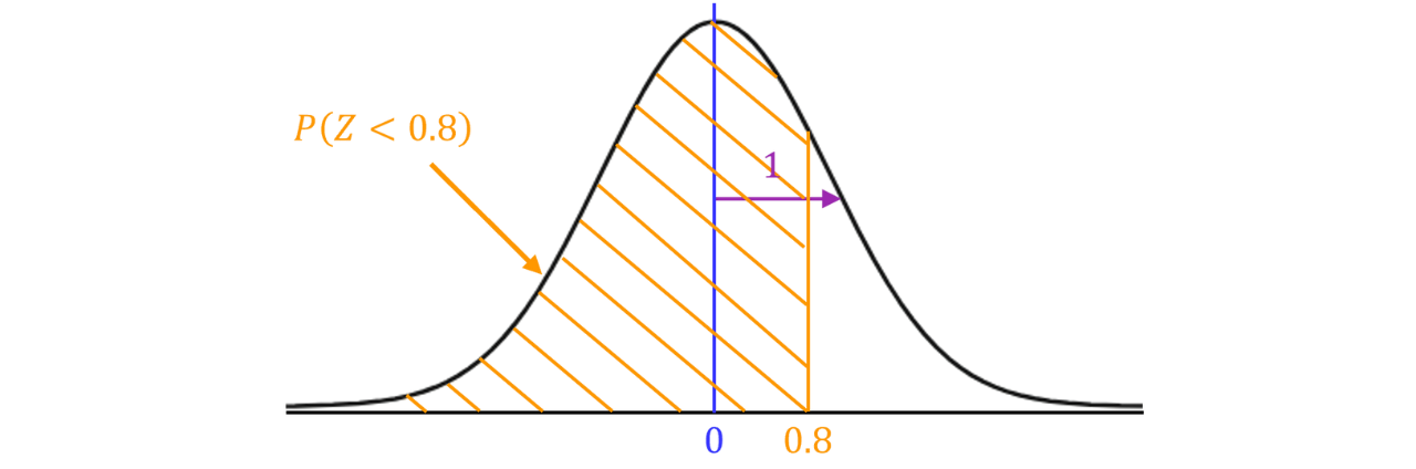
Therefore, using the fact that , we have
b)
Step 1: Apply the transformations to turn the distribution into a distribution.
Note: is the same as as this is a continuous distribution so we do not need to make any adjustments to the inequality.
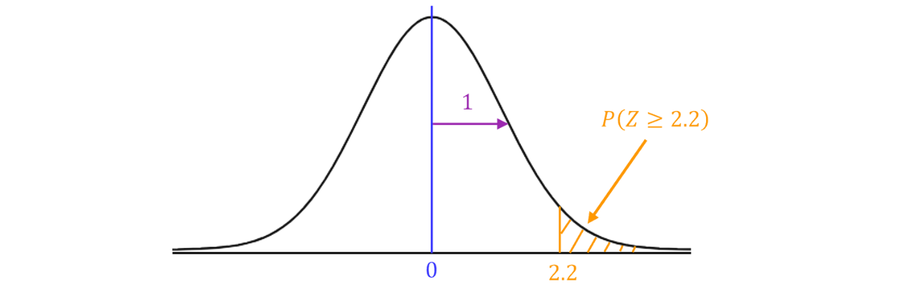
In this case, , and .
Here is a diagram representing the distribution, with , and .
Step 2: Rewrite the probability so that we can use definition of the cumulative distribution function .
Note: Remember that for the cumulative distribution, we need . Currently, we have .
By definition, , which is the area to the left of under the standard normal distribution curve.
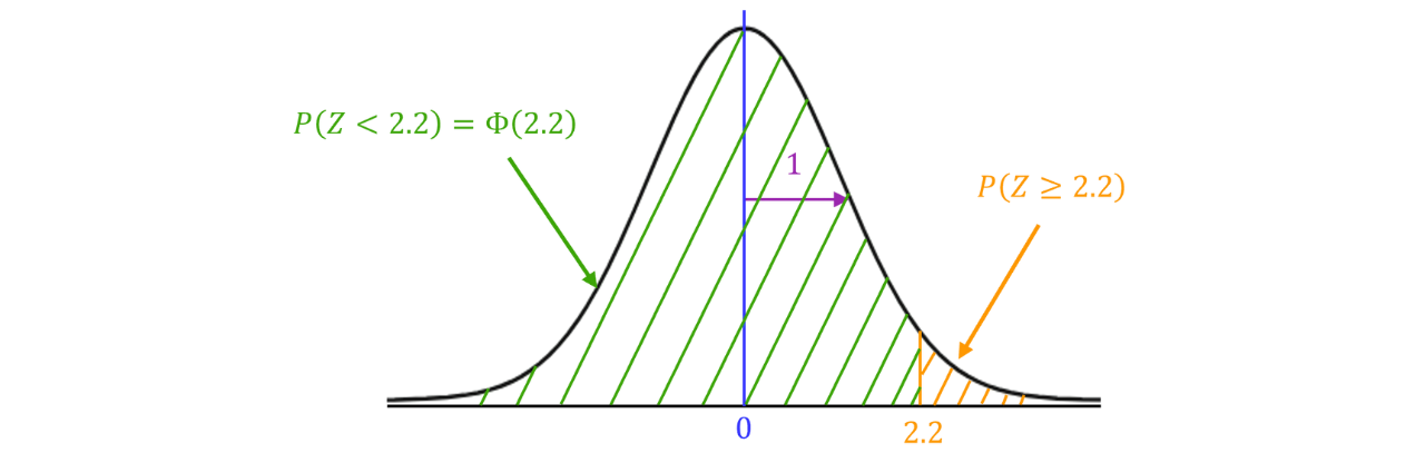
Since the total area under the normal distribution curve is ,
No answer provided.
Example 2:
The times taken, in minutes, for a train to travel from London to Amsterdam are normally distributed with mean and standard deviation minutes. It is given that of the train journeys take less than minutes to complete.
a) Find the value of , giving your answer to the nearest integer.
Step 1: Set up our normal distribution.
Let be the times taken for a train to travel from London to Amsterdam.
The question tells us that of the train journeys take less than minutes to complete. So,
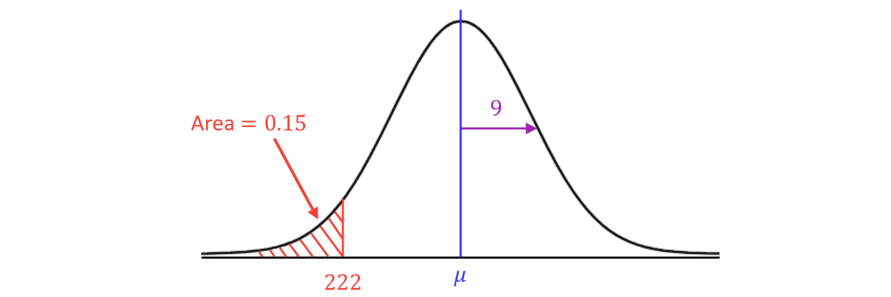
Step 2: Since the mean is unknown, we use transformations to turn the distribution into a distribution.
In this case, and , while is what we're trying to find.
Using the fact that ,
Step 3: Solve for .
First, we apply on both sides, the and will cancel on the LHS.
To evaluate , we go to the inverse normal function in our calculator and input the
area , and .
Multiplying both sides by ,

Therefore, the mean journey time is minutes to the nearest integer.
b) Find the percentage of train journeys which take longer than minutes, giving your answer to significant figures.
Step 1: Use the calculator to evaluate .
Firstly, here’s a diagram representing this distribution and showing the area we want to find.
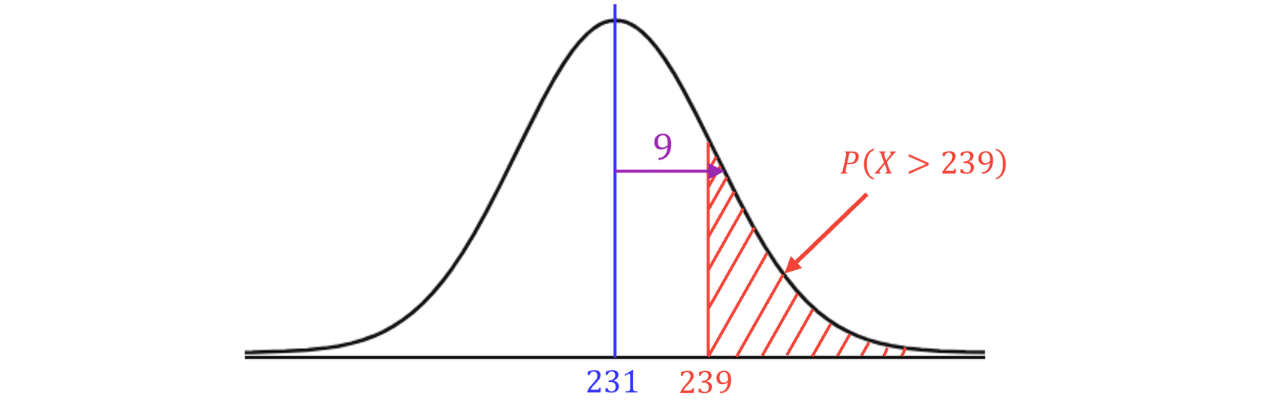
In our calculator, we go to Normal CD, and then input , , lower bound , and the upper bound to be some large number such as . We will find that
Step 2: Convert the probability into a percentage.
To convert to a percentage, we multiply by ,
sf
Therefore, approximately of train journeys from London to Amsterdam take longer than minutes to complete.
A new timetable is implemented, and it is found that the train journey times are now normally distributed with mean minutes and standard deviation . It is given that of the train journeys took between and minutes to complete.
c) Find the value of , giving your answer to significant figures.
Step 1: Set up our normal distribution.
Let be the times taken for a train to travel from London to Amsterdam after the new timetable was implemented.
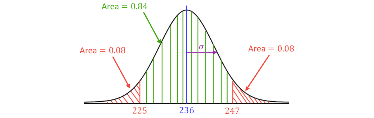
The question tells us that of the train journeys take between and minutes to complete. So,
To use the inverse normal distribution, we need to write a cumulative statement (an area up to a certain value). We could choose the area up to or but finding the area up to is simplest.
Since and are both away from the mean, they are symmetrical about the mean. Therefore, if the middle area is , the end tails are each which means we can write a cumulative statement for as .
Step 2: Since the standard distribution is unknown, we use transformations to turn the
distribution into a distribution.
Here, we will convert
In this case, and , while is what we're trying to find.
Using the fact that ,
Step 3: Solve for .
First, we apply on both sides, the and will cancel on the LHS.
To evaluate , we go to the inverse normal function in our calculator and input the
area , and .
Rearranging for , we multiply both sides by and divide by
Therefore, the new standard deviation is approximately minutes.
No answer provided.
Challenging Question