Rates of Change and Graphs
Neil Trivedi
Teacher

Contents
Rates of Change and Graphs
In real life, quantities are constantly changing. A rate of change tells us how quickly one quantity changes compared with another.
Examples of where we may work with rates of change include:
Distance-time graphs
Velocity-time graphs
Estimating the rate of increase or decrease in values such as population at a given time.
On a graph, the rate of change is found by working out the gradient of the line or curve.
As a reminder, the gradient of a line is found by working out the change in (or change in the variable that lies along the vertical axis) and dividing it by the change in (or change in the variable that lies along the horizontal axis).
We will cover finding the gradient of a curve at a specific point later in this note.
Gradients of Distance-Time Graphs
On a distance-time graph, time (typically in seconds) is plotted on the horizontal axis and distance (typically in metres) on the vertical axis. The gradient tells us how much distance is covered each second, which is the speed of the object.
This is because, as mentioned earlier, the gradient measures the rate of change of a value, so the rate of change of distance is measured by the speed.
Distance-Time Graphs
The gradient of a distance-time graph is the speed of the object.
A horizontal line means the object is stationary (no gradient means no speed).
A negative gradient means it is moving back towards its starting point.
Example 1:
The distance-time graph shows a particle’s journey over seconds.
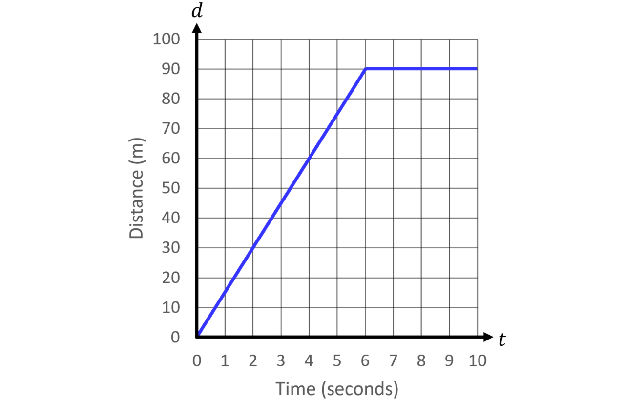
a) Calculate the speed of the particle during the first seconds.
Single Step: Work out the speed by finding the gradient of the line in the first seconds.
We are interested in the part of the graph that’s coloured red.
We need to find change in the distance travelled and divide it by the change in time to get the gradient, which is the speed.
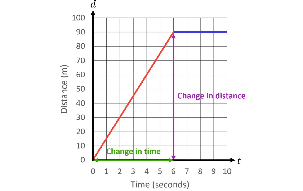
The particle is going from to so the change in distance is The time is from to seconds so the change in time is seconds.
Dividing the change in distance by the change in time, we get a gradient of
Therefore, the speed of the particle during this part of the journey is
b) Describe the motion of the particle between and seconds.
Single Step: Observe the graph and describe the motion.
We are interested in the part of the graph that’s coloured orange.
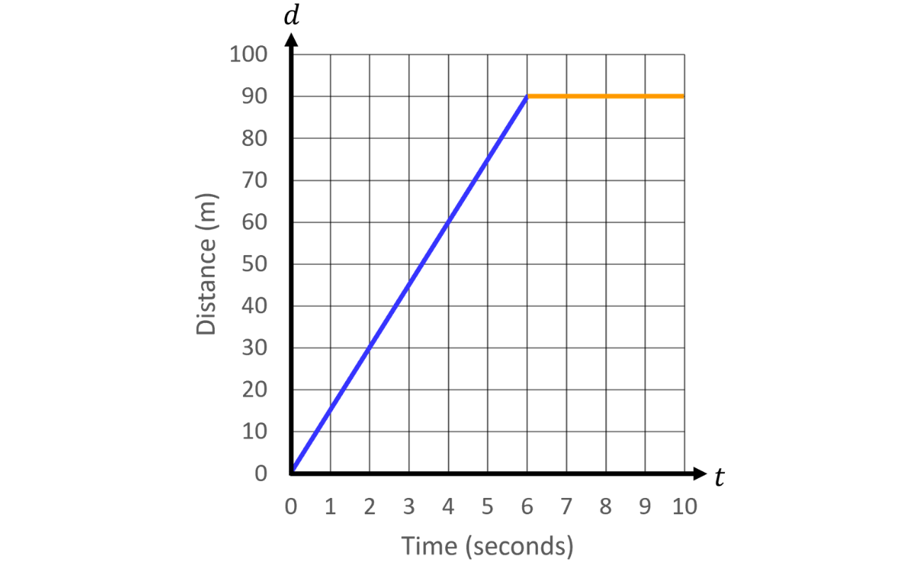
On a distance-time graph, a horizontal line indicates that an object is stationary.
If we were to look at this in terms of gradients, the particle remains at between and seconds, so the change in distance is Therefore, the gradient will be and hence, the speed will be
In an exam, we’d write something along the lines of this:
The particle is stationary at m between and seconds.
Gradients of Velocity-Time Graphs
On a velocity-time graph, the gradient tells us how quickly the velocity changes each second. This is the acceleration.
Velocity-Time Graphs
The gradient of a velocity-time graph is the acceleration.
A positive gradient means the object is accelerating (speeding up).
A negative gradient means the object is decelerating (slowing down).
A horizontal line means the object is moving at a constant velocity (zero acceleration).
Example 2:
The velocity-time graph shows the motion of a motorbike over seconds.
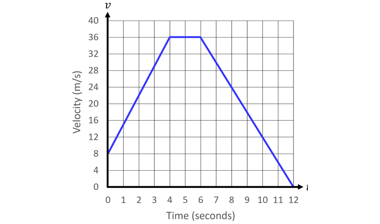
The motion has three parts. Find the acceleration in each part.
Single Step: Find the acceleration in each part by working out the gradients of the lines in these parts.
To illustrate, here are the three parts of the graph shown in different colours.
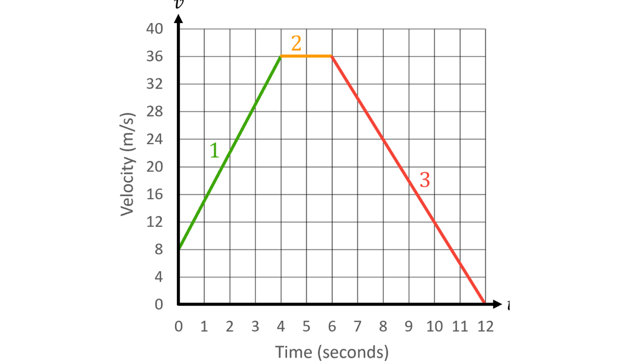
Part (from to seconds):
In this part, the velocity increases from to so the change in velocity is The time elapsed is seconds.
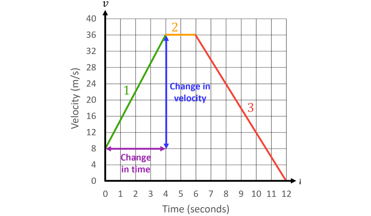
Dividing the change in velocity by the change in time, we get a gradient of
Therefore, the acceleration of the motorbike in this part is
Note: The reason why have chosen these units is because we are measuring the rate in which the speed changes, which is the acceleration.
Part (from to seconds):
In this part, the velocity remains at so it is travelling at constant velocity. This means that the acceleration of the motorbike is
Part (from to seconds):
In this part, the velocity decreases from to so the change in velocity is The time elapsed is seconds.
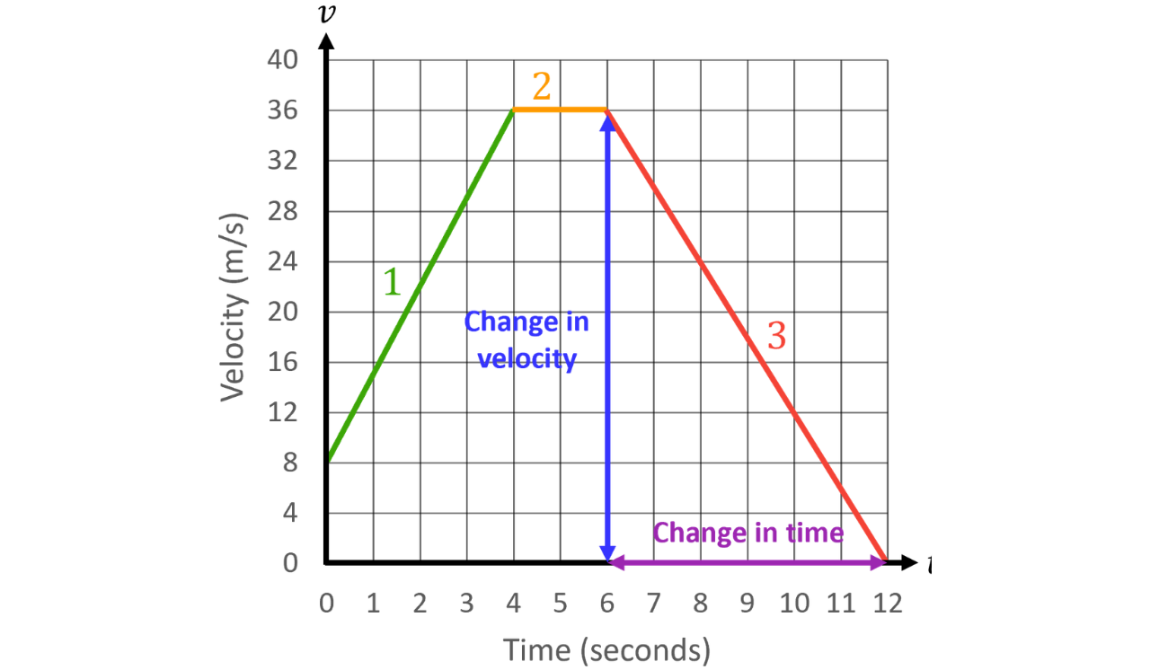
Dividing the change in velocity by the change in time, we get a gradient of
Therefore, the acceleration of the motorbike in this part is
Note: If it asked for the deceleration, the calculation would be the same, but we would change the way we word our final sentence to "The deceleration of the motorbike is
Gradients of Curves
In real life, motion usually involves a changing acceleration, so velocity-time graphs are often curves rather than straight lines. We cannot read the gradient of a curve directly because its steepness is different at every point.
In the previous example, the acceleration instantly changed from to then which is unrealistic.
The next question we must ask ourselves is “how do we find the gradient of a curve?”
To do that, we must use tangents.
The Gradient of a Curve
The gradient of a curve at a point is equal to the gradient of the tangent to the curve at that point.
Remember that a tangent is a straight line that just touches the curve at that one point.
The gradient of the tangent on a curve at a given point gives the instantaneous rate of change, which is the rate at one exact moment. This is because the gradient is constantly changing, unlike a straight line where it is constant.
Example 3:
The velocity-time graph shows the motion of a particle over seconds.
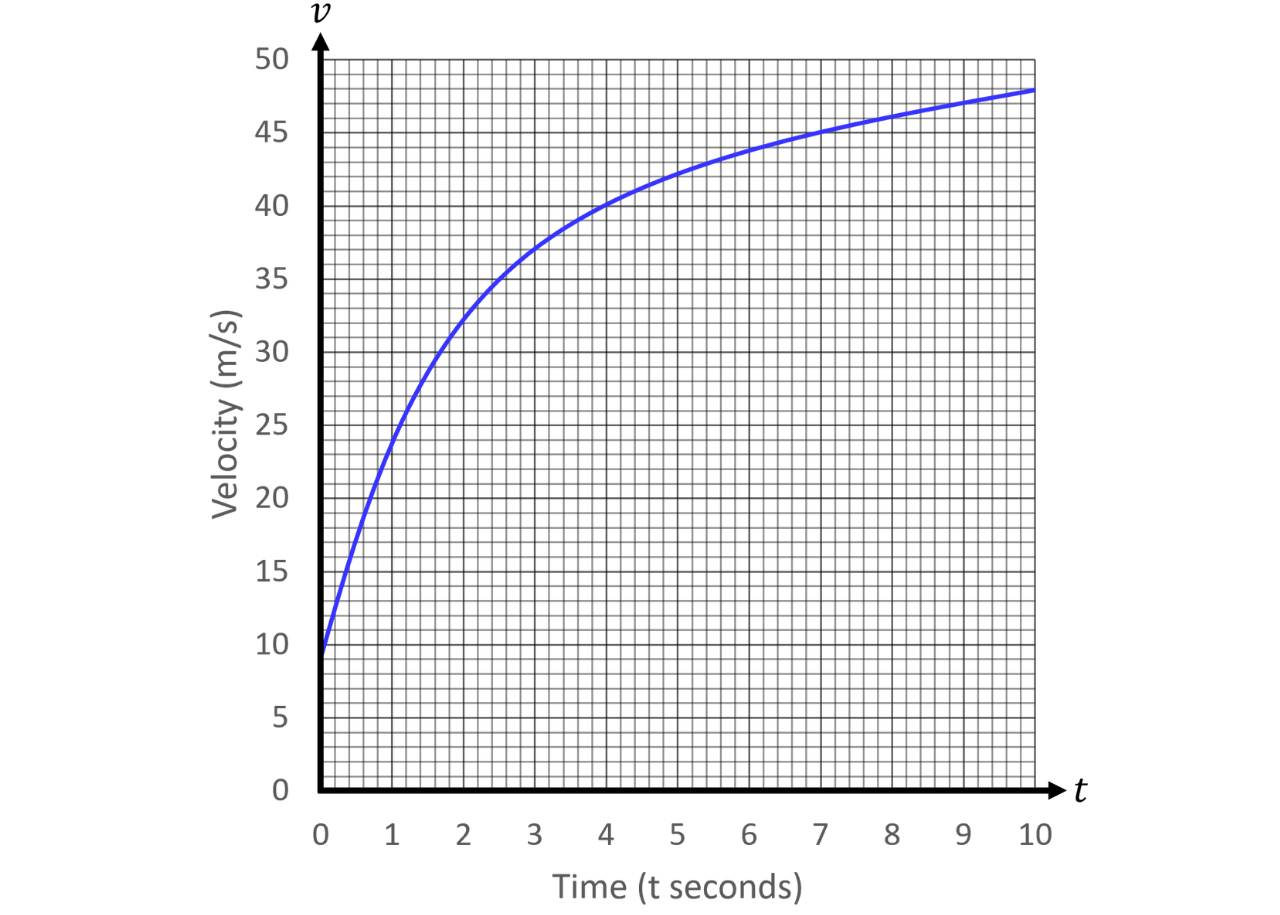
a) Calculate an estimate for the acceleration of the particle when
Step 1: Draw a tangent on the curve at the point where
At GCSE, there is no formal way of finding the equation of a tangent of a curve at a given point, so you will have to do your best to use your ruler to draw the tangent. You are aiming to have an equal gap between the tangent and the curve on each side of the point.
The mark scheme will give a range of answers to allow for student error when drawing the tangent. This is why the question says to estimate the acceleration.
Here is the graph with the tangent drawn at
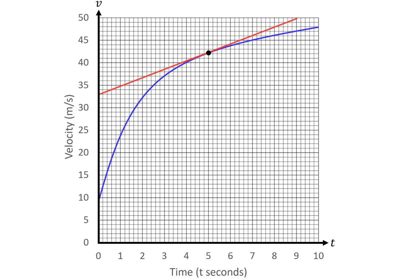
Step 2: Read off two points from the tangent and use these coordinates to find the gradient of the tangent, giving us the acceleration.
The following graph shows two points on the tangent. It also indicates the change in time and the change in velocity between these two points.
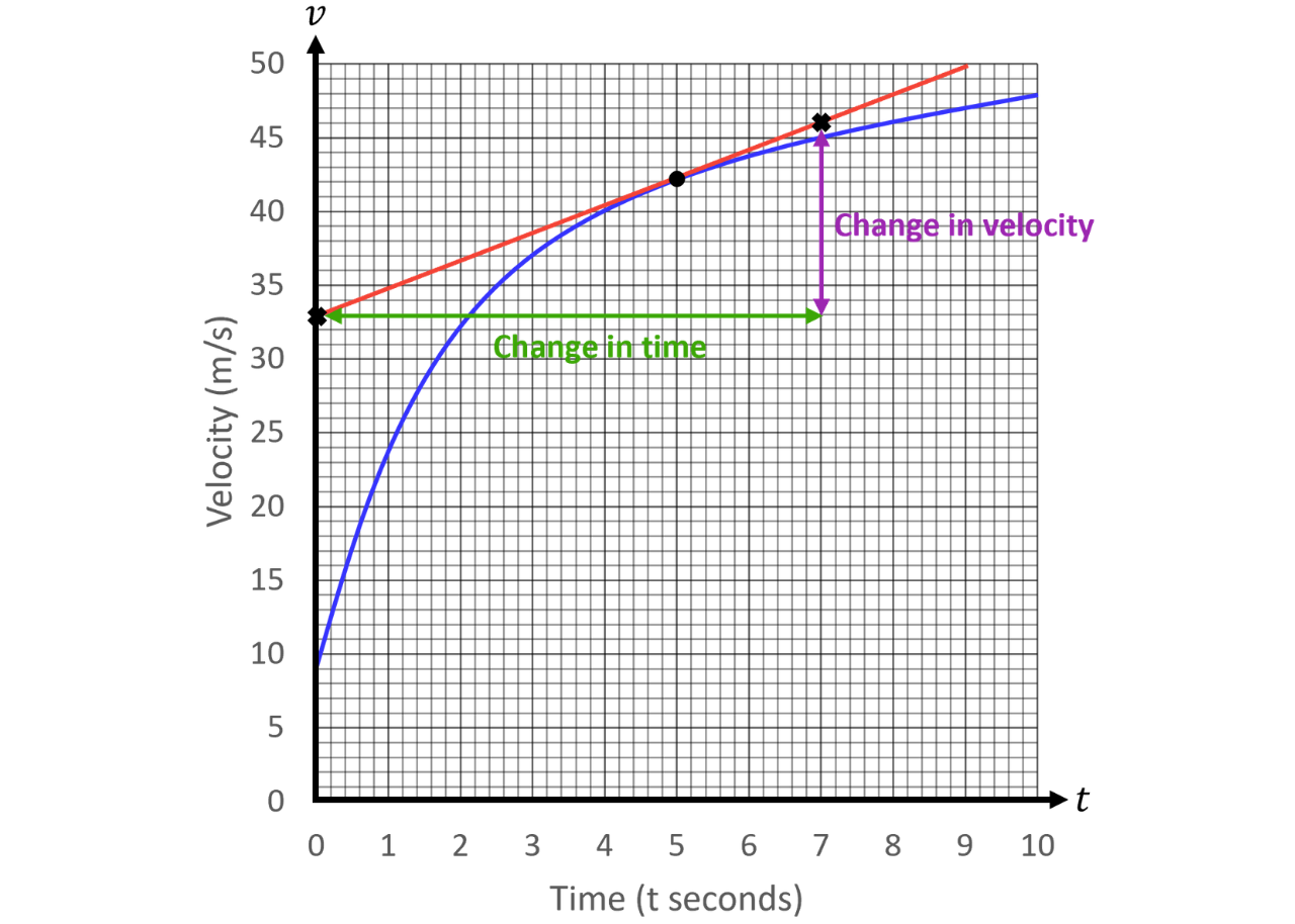
Reading off the graph, we have chosen the points and
Note: When picking two points, you should aim for the points to be as far apart as possible as this reduces errors when reading coordinates.
The change in velocity is and the change in time is seconds.
Dividing the change in velocity by the change in time, we get the gradient of the tangent to be
Therefore, the acceleration of the particle at is approximately to significant figures.
b) Work out the average acceleration of the particle between and
This question is asking about the average acceleration in those seconds, which is the average rate of change in velocity between and
The way we think about this problem is we say “at the beginning, our velocity was and after seconds, our velocity was What is the acceleration between these two points?”
So, we would draw a straight line that joins the two points on the curve and then work out the gradient of the line.
Step 1: Draw a straight line on the graph, joining the point at to the point at
Here is the graph with the straight line drawn. It also indicates the change in velocity and the change in time.
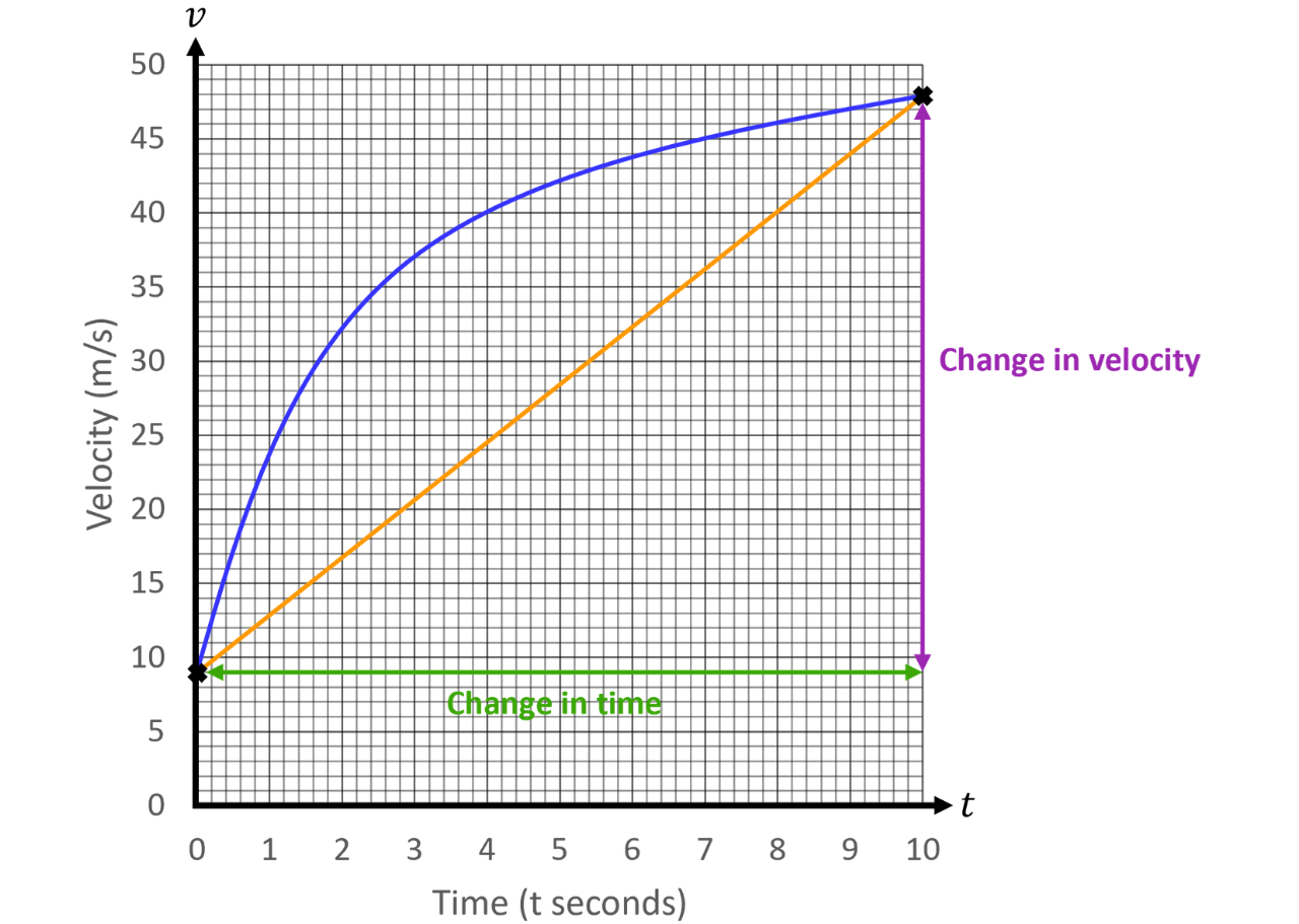
The two points that are joined are and
Step 2: Find the gradient of the straight line, which will give the average acceleration of the particle between and
The change in velocity is and the change in time is seconds.
Dividing the change in velocity by the change in time, we get the gradient of the line to be
Therefore, the average acceleration of the particle from to is
Finding Distances from Velocity-Time Graphs
From a velocity-time graph, we can find the acceleration of the object by working out the gradient.
We can also find the distance travelled by working out the area under the graph.
If the graph is made up of different shapes, we split the area into separate shapes like rectangles, triangles or trapezia. We then find the area of each shape and add them together to get the total distance travelled.
The Area under a Velocity-Time Graph
The area under a velocity-time graph is the distance travelled.
Example 4:
Find the distance travelled in this velocity-time graph.
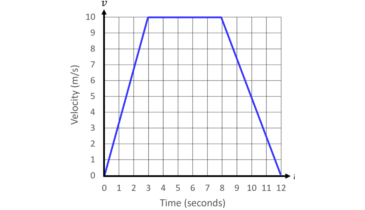
This graph forms a trapezium, so we just find the area of the trapezium to get the distance.
Single Step: Find the area of the trapezium.
The area of a trapezium is given by
Area
where and are the parallel lengths and is the height.
Here is the trapezium formed by the area under the velocity-time graph with all the relevant lengths labelled.
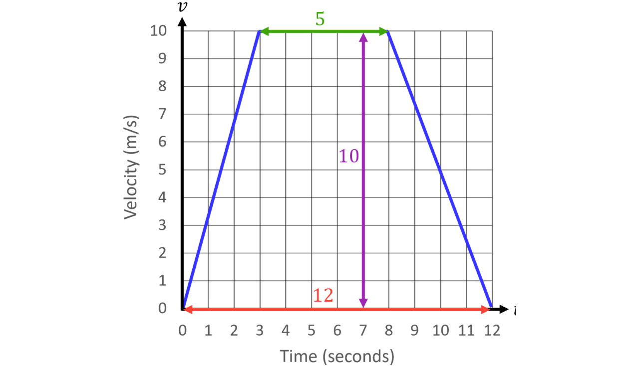
Here, the parallel lengths of the trapezium are and while the height is
So, the area is
Therefore, the distance travelled is
Finding Distances on Curved Velocity-Time Graphs
When a velocity-time graph is a curve, we cannot find the exact area/distance under the curve. Instead, we estimate the area by splitting it into vertical strips, such as triangles and trapezia.
Here is an example showing why we estimate the area rather than finding the exact area.
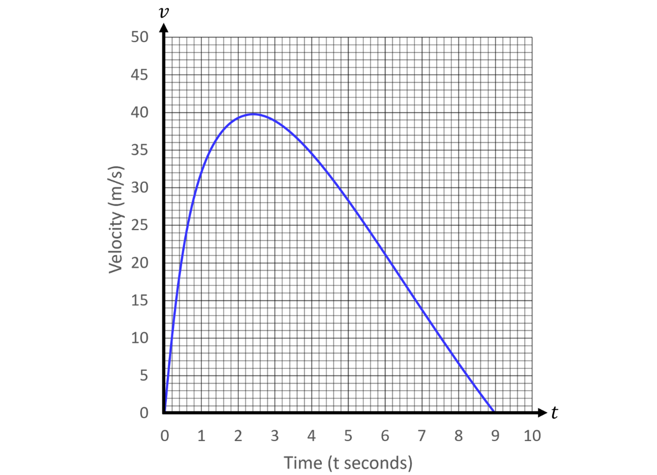
Let’s split this graph into strips of equal width.
When we split the area under the curve into two triangles (labelled and and one trapezium (labelled some of the area under the curve may be missed out (shown shaded in green). In this example, more area is missed out than added above the curve, so the estimate is an underestimate.
Notice how the top edges of strips and are below the curve but the top edge of strip is only slightly above the curve. The fact that strips and are so far below the curve counters the fact that strip overestimates the area ever so slightly.
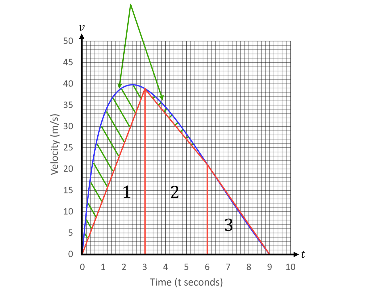
In other cases, the strips may include more extra area above the curve than the area they miss out below the curve. This would make the estimate an overestimate.
To find the exact area under a curve, we would use a process called integration, which is covered in A-level Maths.
Example 5:
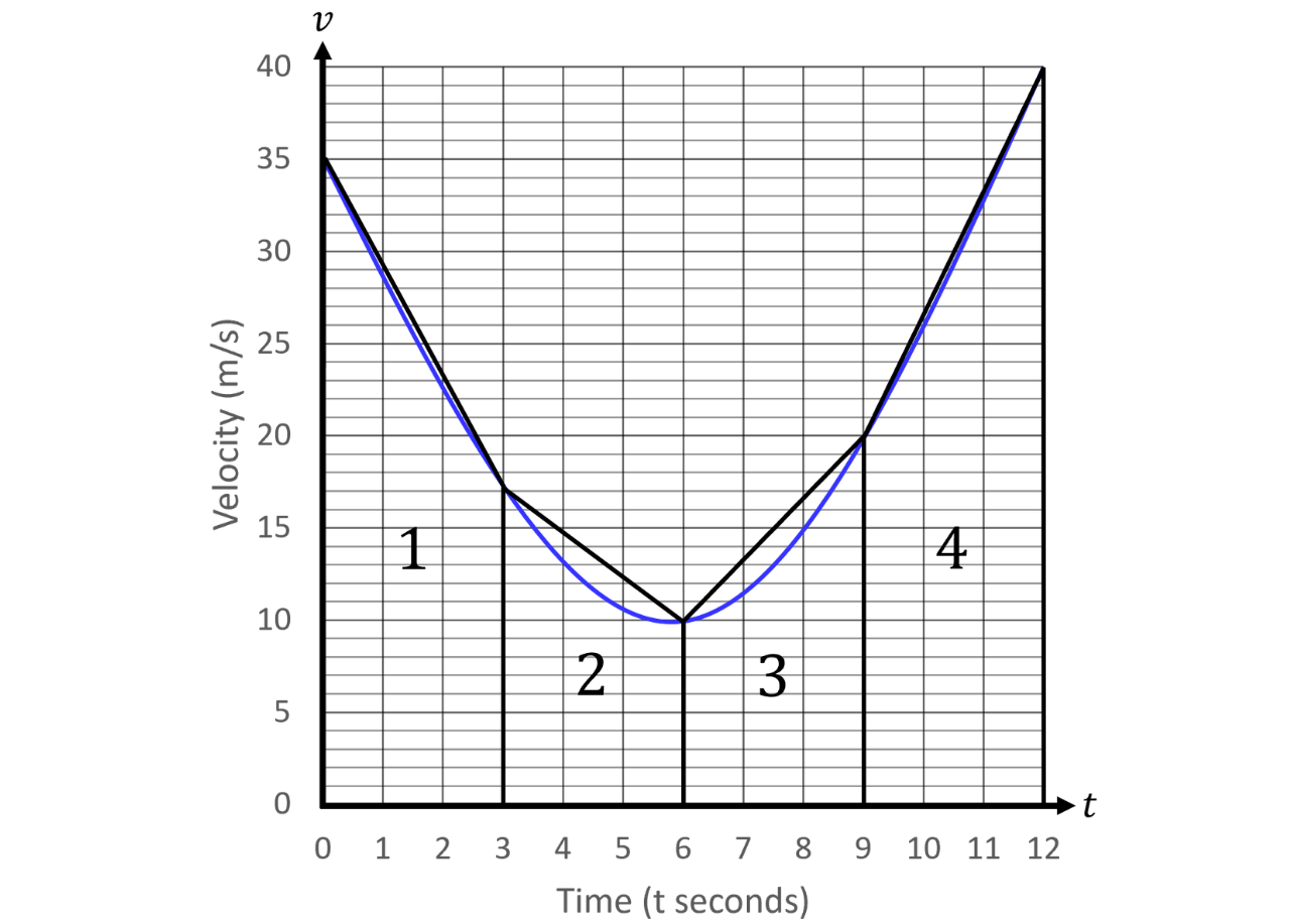
Here is a velocity-time graph, showing the motion of a car.
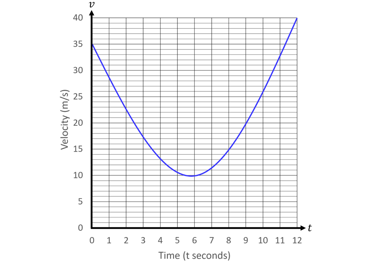
a) Estimate the distance the car travelled using strips of equal width.
Step 1: Split the area under the curve into strips of triangles and/or trapezia.
The motion is over seconds, so the strips will cover seconds each. We get the following graph with the strips added on.
Step 2: Find the area of each strip.
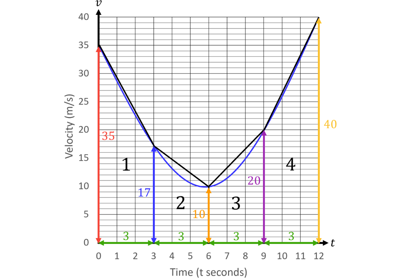
Each strip is a trapezium. The “height” of each strip is measured along the horizontal axis, which is for each strip. The two parallel sides are measured along the vertical axis. Reading off the graph, we get the following lengths and areas.
Strip
Area
Strip
Area
Strip
Area
Strip
Area
Step 3: Add the areas of the strips together to get an estimate for the distance covered by the car.
Therefore, an estimate for the distance covered by the car is
b) Is your estimate for the distance an overestimate or an underestimate?
Single Step: Observe the graph and identify added or missed areas.
Here is an annotated graph showing the areas that are missed out under the curve or the extra areas above it that are included by the strips.
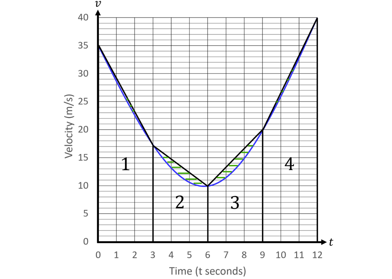
From the graph, we can see that the strips cover more extra area above the curve than the area they miss out below the curve. This is especially clear for strips and
Therefore, the estimated area under the graph is greater than the exact area under the curve.
In the exam, you would phrase it like this:
“The top edges of the strips lay above the curve, so the estimate for the distance travelled by the car is an overestimate.”
Practice Question