Graphs
Brook Edgar
Teacher

Contents
Explainer Video
Graphs
After an experiment, we want to plot a graph of our results to determine relationships. We aim to plot a linear graph of the form: .
We can then determine the gradient and the y-intercept of the graph. See example below:

The equation of the line in the example above is then, .
If the line of best fit does not follow the relationship, and is a curve, to find the gradient at a point, you draw a tangent to the curve at that point and find the gradient of that line.

For example, to determine the gradient of the graph above at , draw a tangent to the curve at the point of interest and calculate the gradient of that tangent.

Remember: Ensure your pencil is sharp when drawing the line of best fit, and that the triangle you draw to find the gradient is as large as possible to reduce the % uncertainty in your results -> rule of thumb is to aim for your triangle to be larger than on one side.
We need to be able to calculate the percentage uncertainty from graphs. To do this, draw the line of best fit and then a "worst-case" line of best fit (the steepest or shallowest line that still passes through all error bars, if present). Calculate the two gradients and use the equation:
-> The modulus bars mean that the percentage uncertainty is always positive.
-> You need to learn this equation.

Alternatively, the percentage uncertainty in the -intercept can be found:
Plotting graphs
Often relationships are non-linear, so we need to transform them to a straight-line form in order to plot a graph.
For example, if water is displaced by an amount in a tube, the time period, , varies by, . If we want to determine from the results we need to find out what to plot on our graph.
We want the equation in the form , where some form of is on the -axis and some form of is on the -axis as they are our dependent and independent variables.
and are not ideal, so the first step is to square the whole equation and then rearrange into the form .
->

Logarithmic Graphs
Many relationships in Physics involve exponentials, such as that for a capacitor . To plot a graph of these relationships, we need to use log rules to make the equation into the form . The rules apply to both logs to the base , , and natural logarithms, to the base , .
->
-> , therefore
-> , This is a useful rule and used often.
Often is just written as .
->
->
For example, if the relationship is and measurements of and are taken, what would we plot to solve for the unknowns and ?
Firstly we need to take natural logs of both sides of the equation to make the equation into the form of .
Use log rules:
->
->
Rearrange to fit the form :

Worked Example
is the amplitude of the pendulum.
is the amplitude over swings.
is a constant known as the damping factor.
If the axes are as shown in the graph, how would you determine ?

Answer:
Want the equation to be linear, in the form , where some form of is on the -axis and some form of is on the -axis.
Take the natural log of both sides:
Use log rules to separate terms
->
->
Rearrange to fit the form :
->
Gradient,
The question asks to find :
->
->
Proving Relationships
To prove a relationship you need to take a minimum of three different readings from the graph.
For example, looking at the graph below one might think it follows the inverse square law, .

To prove this, we take three different readings to determine if is in fact a constant.
Different values after only two times. We can stop here as it is clear is not constant. The line does not follow the inverse square law.
What if it is a reciprocal graph following the relationship, .
Different values, after only two times. is not constant. It is not a reciprocal graph.
What about exponential decay?
To prove this, we need to show that the y values drop by the same factor over equal increases in the -axis.
As increases from (up by ), the value drops ,
As increases from (up by ), the value drops ,
As increases from (up by ), the value drops ,
The graph shows exponential decay as the y values drop by the same factor of every time the value increases by .
Worked Example
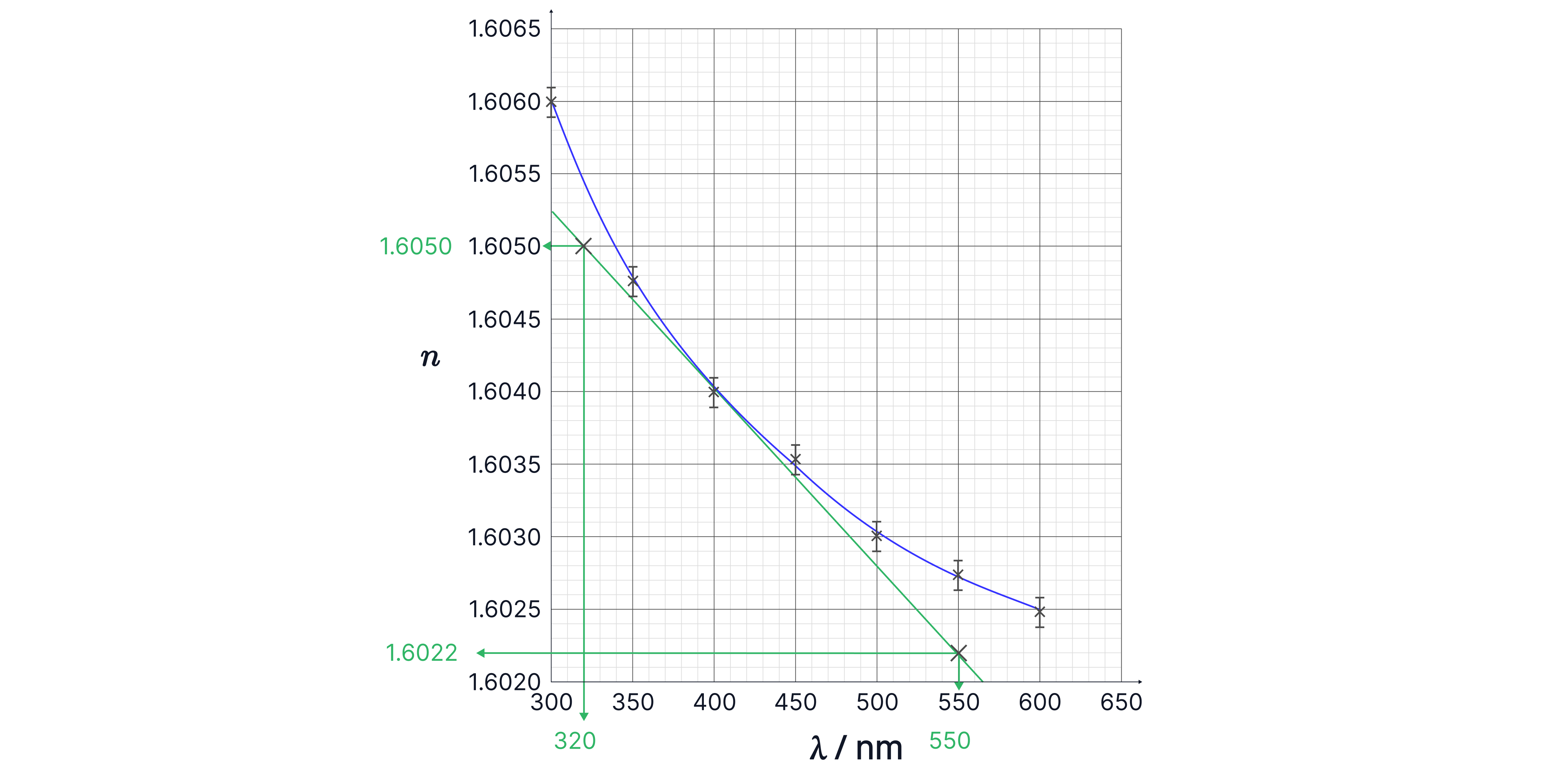
The graph shows how the refractive index, , of a type of glass varies with wavelength of light. One student suggests that it resembles the decay of radioactive nuclei, showing half-life behaviour. Comment if they are correct.

Answer:
If it is an exponential relationship, the value drops by the same factor over an equal interval in the –axis.
, value decreases ,
, value decreases ,
, value decreases ,
Equal increases in -axis have the same factor of decrease on the -axis of , to three significant figures, so the graph does show exponential decay.
Oscilloscopes
Oscilloscopes have two controls that you need to know how to read and manipulate:
-gain in volts per division, usually .
Time-base in time/division, usually .

Below the time-base setting is off, and the voltage is .

If we connect the oscilloscope to a battery, with the time-base setting still off:

If we turn the time-base setting on, then we see a flat line, as a battery is a DC source.

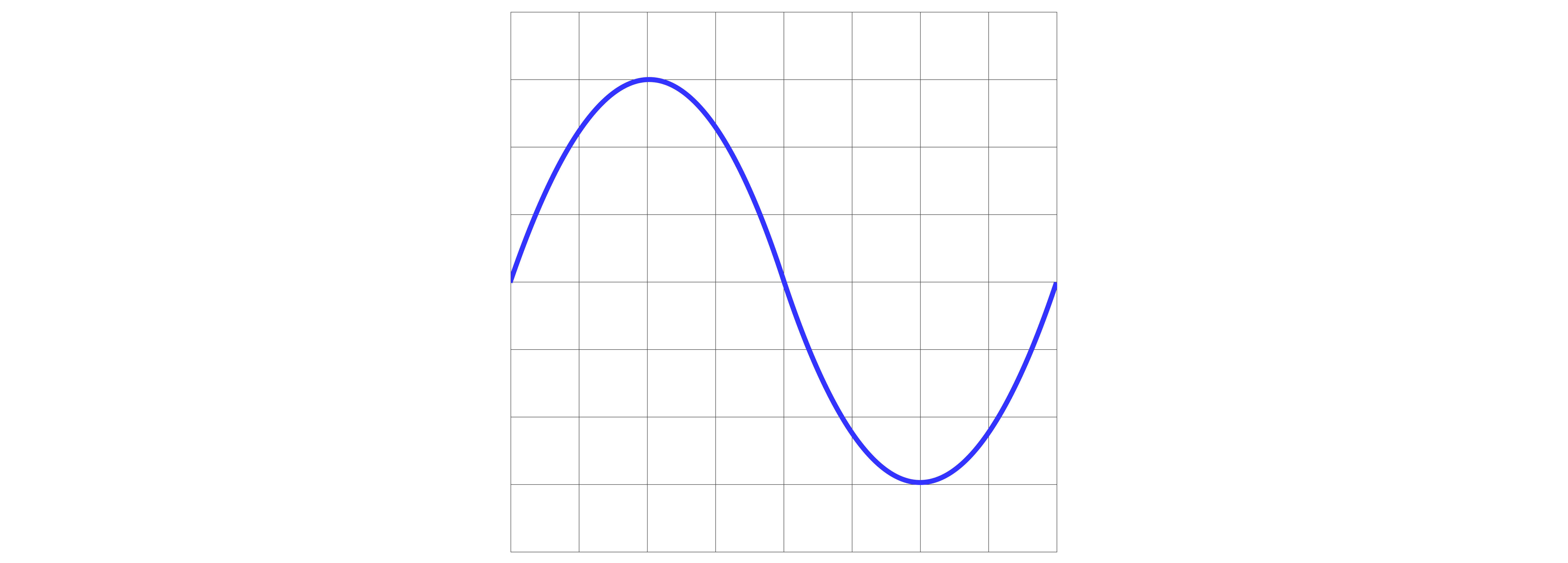
If we had connected the oscilloscope to a AC source with a peak voltage of we would see the below:

If the voltage of the source is unknown and we need to use the oscilloscope to determine the voltage, we would want the wave on the screen to cover as much of the screen as possible to reduce the percentage uncertainty in our results. To do this, we would decrease the -gain setting. Instead of which covers a total of six boxes on screen, as we want the wave to cover a total of eight boxes on screen, we would change to .
If the frequency of the source was unknown and we wanted to use the oscilloscope to determine this, we would want multiple waves on the screen, not just one. We would need to change the time-base setting. We would , for example, increase the time base setting from which allows one wave across eight boxes to to allow two waves across the eight boxes.
Worked Example
An AC source with a peak voltage of with time-base setting on.
Calculate the frequency.
Time-base setting: .
 Answer:
Worked Example
The image on the oscilloscope is when the -gain is set at per division and a time-base setting of per division.

Which is observed when the -gain is set to per division and the time-base setting to per division?

Answer:
Vertical scale (Y-gain):
Y-gain is volts per division.
Changing from 2 V/div → 4 V/div means each vertical division now represents twice as many volts.
For the same signal voltage, the height (in divisions) on the screen therefore halves.Horizontal scale (time-base):
Time-base is time per division.
Changing from 10 ms/div → 20 ms/div doubles the time shown per division.
Over the same screen width, you now display twice as much time, so twice as many cycles fit on the screen. The waveform looks more compressed horizontally (each cycle occupies half as many divisions).
Combining both changes: half the vertical height and twice as many cycles across the screen → this matches trace D.
Practice Questions
How do we find using the graph below?

-> Check out Brook's video explanation for more help.
Answer:
It can be shown that decreases exponentially with .
Show that , the decay constant, for this process is using the graph below.

-> Check out Brook's video explanation for more help.
Answer:
Use two points on the graph, plug into the equation, , and solve for the decay constant.